Jamie Bernardi

Introduction

Value learning algorithms usually centre around the infinite horizon Bellman equation. When we make estimates of the value of an action, we are estimating the value of the entire future given a current state and proposed action. However, such value learning approaches are notoriously unstable.

Finite-Horizon Temporal Difference methods were recently reintroduced to shorten the time step horizon where value is being maximised over, to a finite number of steps. The authors boast proven training stability and higher predictive power, by taking this approach. We additionally found them to converge in fewer time steps. A finite number of steps can approximate an infinite number of steps arbitrarily well, though most toy RL problems need far fewer steps than infinity to realise the value of an action; e.g., reward feedback is usually much more rapid.

Recently I found use for FHTD methods whilst working on a project investigating pessimistic agents – with thanks to Michael Cohen for pointing this paper out. This is a very useful method that is not circulating as much as I’d expect given its benefits.

In this post I’ll present arguments for and against, provide an implementation and present an empirical comparison between FHTD and infinite Bellman value learning.

Background – infinite Bellman equation

In Q-value learning, a function Q(s, a) is learned. This is an estimate of the value (expected accrued reward) over the entire future, by taking action a from state s. Some discount factor gamma bounds it to a finite number, in practice. Below is the update definition; given a state and action at time step t, and observed next state and reward, the new Q value is updated toward the target, by adding the “temporal difference” to the current Q value.

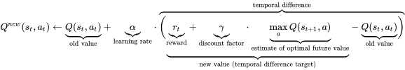
Agents usually follow a policy of taking the action that maximises Q(s, a); action = argmax_a’ ( Q(s, a’) ).

Introducing the Finite Horizon

Converse to the infinite Bellman equation, FHTD learns functions that estimate the value, or expected accrued reward, over a fixed number of future time steps. This results in a new update function, one for each time step h, as below.

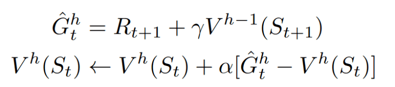
In English:

• G^{h}_t is the estimate of the value accrued in h steps from the current time step t.
• R_{t+1} is the reward obtained in stepping to state s_{t+1}
• Gamma * V^{h-1}(S_{t+1}) is the discounted, estimated value accrued in h-1 steps from the next state, s_{t+1}.

The estimate G, of the value accrued in h steps from the current time step, is has the value estimate V^{h}(S_t) subtracted from it to construct the temporal difference (analogous to Bellman update above).

In Q learning, the value V^{h} would be estimated by taking max_a’ ( Q^{h}(s, a’) ). Agents typically act by taking the argmax over actions for the value estimate furthest in the future (h=H).

A word on stability

As we saw in the Bellman equation, new values of Q are learned by bootstrapping off itself. The temporal difference is calculated with the reward, and a call to the very same Q function being updated, with the next state as its argument. This bootstrapping the source of value learning’s instability.

In FHTD, each V^{h} is a separate estimator of value – with its own parameters – for every horizon h. Therefore, to paraphrase the abstract, because each value function V^{h} calculates its temporal difference with the previous estimator V^{h-1} rather than itself, fixed-horizon methods are immune to the stability problems that infinite horizon learning faces.

Intuition for convergence

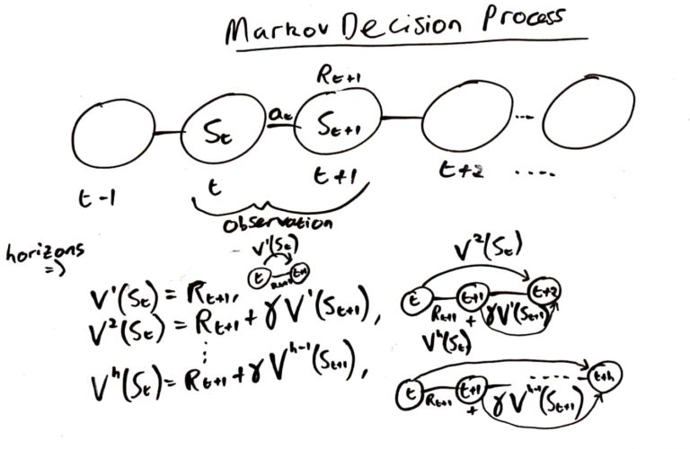
An inductive intuition is useful at this point. When h=1, V^{1} is just the estimate of the immediate reward (as V^{0} is always 0 – there is no reward to accrue in 0 time steps). So V^{1} can converge trivially, from observations of immediate rewards received. Therefore V^{2} is the reward obtained in stepping from horizon 1 to 2 (simply the observed rewards), added to the discounted value estimate of the 1-step horizon at state 2 – V^{1}(s_2). We said V^{1} was simply the immediate reward, and we can intuit that that should converge. Therefore when a good estimate of V^{1} is learned, V^{2} will follow suite. That argument is followed inductively to an arbitrary number of time step horizons.

It is worth considering what it means that each of the N horizons are updated from a single state, action, reward, next state observation. This algorithm does not collect a trajectory of observations, nor try to explicitly learn a trajectory; doing that would not be able to generalise an observation of step t->t+1 to all horizons h-1->h, and we would be learning less about the dynamics of the environment.

Pros & Cons

The authors list two benefits, and I observe a third benefit:

• Higher training stability; because none of these time step estimates bootstrap from themselves (rather, they bootstrap from the previous horizon), they learn more stably. In fact, the authors offer a proof of convergence – a rare thing indeed!
• Higher predictive power, i.e. the ability to estimate how much value will be accrued in N steps’ time, rather than 1 function that estimates the value of the entire future.
• Converges in fewer time steps; whilst I haven’t analysed this in depth, it makes intuitive sense that each estimator is bootstrapping off a value estimate that converges much faster than the infinite value estimator. Therefore, fewer erroneous updates are made during the early stages of the training process when the future (infinite) Q estimate is unstable, relative to the n-step horizon value estimate where n << infinity.

Working around additional computation

The downside of this method is that it requires an additional value function for every time step horizon you wish to estimate. The authors list some ways to combat this.

• Parallel updates; the algorithm updates every horizon on a given observation, using the frozen previous-horizon estimate to bootstrap from. Therefore each estimator could be updated on a separate thread or processor, which may be more efficient depending on the size of the update taking place.
• Shared weights; have a single network with H outputs predict the H horizons as, again, updates can happen in parallel.
• n-step bootstrapping; instead of estimating H=10 steps with h = {1, 2, …, 10}, achieve the same horizon with fewer estimators h={1, 5, 10} with Multi-step Fixed Horizon TD prediction (as-per paper). This saves on storage and computation, but reduces predictive power and increases the variance per update. It’s achieved by updating on n-step sub-trajectories, instead of a single observation.

We didn’t approach any of those in our implementation, as we were not performance constrained in the finite state Q Table setting I have used FHTD in so far. Here, updates are very simple, and don’t involve e.g. gradient descent (see implementation).

A use case – inductive proofs

One motivation for implementing the finite step analysis was for a proof. We initially investigated making an inductive proof, namely:

• Prove a property for k=1 (horizon 1)
• Assuming the property holds for k=n, prove for the next step, k=n+1
• Induce that property is true for all integers k={1, 2, 3, …}

Looking ahead to a finite number of future time steps is an ideal use case for finite horizon Q Learning. As FHTD is underpinned by a proof of convergence, any modifications to value learning could be considered under the finite horizon framework to prove properties about that modification’s convergence. This avenue didn’t prove fruitful for us, but it could be a useful tool for other researchers.

Implementation details

With thanks to one of my collaborators Peter Barnett, who first parsed the algorithm into our codebase, we provide a working, minimal agent for FHTD Q learning.
Bear in mind this doesn’t mention any of the three tricks the authors propose for more complicated environments, rather serving as a conceptual starting point.
Adapted snippet:

import numpy as np

num_horizons = 5
# 5x5 gridworld with 4 actions
q_tables = np.zeros((5 * 5, 4, num_horizons))
# history = [(state, action, reward, next_state, done), ...]

def update(self, history, lr=1., gamma=1.):
    """Update a finite horizon Q Table"""
    for state, action, reward, next_state, done in history:

        # Note, Q_0 is always 0 and should not be updated.
        #  There is 0 reward to accrue in 0 time steps 
        for h in range(1, num_horizons + 1):
            # Estimate V_(h-1)(s_(t+1)): the reward accrued in h-1 steps
            # from the next state
            if not done:
                future_q = np.max([
                    q_tables[next_state, action_i, h - 1]
                    for action_i in range(num_actions)])
            else:
                future_q = 0.

            # Bootstrap the V_h value off the future value estimate for the
            # next state, added to the reward received in getting to that
            # next state
            q_target = reward + gamma * future_q

            # Update the V_h estimate towards the future estimate
            q_tables[state, action, h] += lr * (
                    q_target - q_tables[state, action, h])

Results

I ran a quick analysis in a finite state environment – originally intended for an experiment investigating pessimistic agents – to support the claims in this post. Some features of the environment are a little particular, namely:

• The agent is an ask-for-help agent; it queries a random, safe mentor policy. This has the same effect as a rollout with random steps, until Q Table values initialised at 0 have exceeded a Q Table initialised at 1.
• The environment has “cliffs” around the edge, where an episode is ended and 0 reward scored. It’s been empirically demonstrated that these states are never encountered.

Otherwise, the environment has stochastic state transitions (expected state as per action with 60%, other 3 states share the remaining 40% randomly), and rewards are Gaussian distributed where the mean is the normalised x-coordinate, standard deviation of 0.1. You can regenerate this plot with the code.

Conclusion

Finite-Horizon Temporal Difference updating is proven to be more stable, with more predictive power, and is shown to converge faster than infinite Bellman updating. The underpinning proof makes it an ideal candidate for inductive proofs about modifications to value learning. I hope to see it utilised more commonly in value learning RL experiments, which are typically fraught with instability, due to the ‘deadly triad’ of off-policy updating of a self-bootstrapping function approximator for the Q value.